Testbench Quickstart

This describes how one can use datapipe-testbench to make one or more studies.

Terminology

• Experiment: describes one configuration that is to be later compared. It is associated with a single InputDataset, and is processed into a set of metrics.

• Study: a comparison of multiple experiments, with the output being a set of plots and verification checks.

The idea is that you can generate metrics for each experiment, and store them in the same place. Later, you can choose from pre-existing metrics and make many comparison studies.

Generating Metrics for one or more Experiment

First set up your input information and choose which benchmarks you will be comparing later. Note that you need to include all benchmarks that you might want to study in the future, and for each benchmark you need to provide the required input data (use print_benchmark_info() to see what is required for your benchmark).

In this example, we will use only one benchmark: benchmarks.dl1.PixelIntensityResolutionBenchmark, which requires the dl1_images input to be defined.

from pathlib import Path

import matplotlib.pyplot as plt

from datapipe_testbench import (
    InputDataset,
    benchmarks,
    generate_all_metrics,
    print_benchmark_info,
    run_comparison_study,
    visualize_comparison_study,
)

# set to where you store metrics
EXPERIMENTS_PATH = Path("~/testbench/experiments/").expanduser()

# set to where you store comparisons
STUDIES_PATH = Path("~/testbench/studies").expanduser()

Choose the list of benchmarks to generate metrics for:

Note that when we construct the benchmark, we can specify options. For example, benchmarks.dl1.PixelIntensityResolutionBenchmark has an option to specify the chunk_size and max_chunks to limit how many events we process, which can be handy when debugging. Here we just use the default, which is to process all events in the file.

benchmark_list = [
    benchmarks.dl1.PixelIntensityResolutionBenchmark(),
    benchmarks.dl1.HillasIntensityResolutionBenchmark(),
]

We can also see some information about these benchmarks, such as what inputs they require. Here, we see tht we will need to set both dl1_images and dl1 in all InputDataset we use.

for benchmark in benchmark_list:
    print_benchmark_info(benchmark)

image resolution
----------------------------------------

Benchmark pixel-wise intensities at the DL1 level, before cleaning.

Input Files Required for Metric Generation:
 * dl1_images

Output Metrics:
 * dispersion          : dl1_images/image_dispersion.asdf
 * bias                : dl1_images/image_bias.asdf
 * resolution          : dl1_images/image_resolution.asdf

hillas_intensity resolution
----------------------------------------
Benchmark post-cleaning Hillas intensity.
Input Files Required for Metric Generation:
 * dl1

Output Metrics:
 * dispersion          : dl1/hillas_intensity_dispersion.asdf
 * bias                : dl1/hillas_intensity_bias.asdf
 * resolution          : dl1/hillas_intensity_resolution.asdf

Next you should define an InputDataset for each experiment, providing an input file for all inputs required by the benchmarks you have selected. In this case, our input files have both DL1 parameters and images and enough stats for both benchmarks, so we use the same file for each. However, that is not always the case: sometimes you want to use a higher-stats input file for dl1 to get better results.

DATA = Path("~/Data/Example").expanduser()

prod5b_dark = InputDataset(
    name="Prod5b-dark ctapipe-0.26.1",
    dl1_images=DATA / "prod5b_dark_gammas_with_images.dl1.h5",
    dl1=DATA / "prod5b_dark_gammas_with_images.dl1.h5",
)

prod6_dark = InputDataset(
    name="Prod6-dark ctapipe-0.26.1",
    dl1_images=DATA / "prod6_dark_gammas_with_images.dl1.h5",
    dl1=DATA / "prod6_dark_gammas_with_images.dl1.h5",
)

prod6_moon = InputDataset(
    name="Prod6-moon ctapipe-0.26.1",
    dl1_images=DATA / "prod6_moon_gammas_with_images.dl1.h5",
    dl1=DATA / "prod6_moon_gammas_with_images.dl1.h5",
)

input_datasets = [prod5b_dark, prod6_dark, prod6_moon]

Finally, we will define which benchmarks we want to compute metrics for, and generate them.

_ = generate_all_metrics(
    input_dataset_list=input_datasets,
    benchmark_list=benchmark_list,
    experiments_path=EXPERIMENTS_PATH,
    skip_existing=True,  # don't re-process files that we have already processed
)

Processing:
  * Benchmarks: ['image resolution', 'hillas_intensity resolution']
  *     Inputs: ['Prod5b-dark ctapipe-0.26.1', 'Prod6-dark ctapipe-0.26.1', 'Prod6-moon ctapipe-0.26.1']

Prod5b-dark ctapipe-0.26.1 -- image resolution

Prod5b-dark ctapipe-0.26.1 -- hillas_intensity resolution

Prod6-dark ctapipe-0.26.1 -- image resolution

Prod6-dark ctapipe-0.26.1 -- hillas_intensity resolution

Prod6-moon ctapipe-0.26.1 -- image resolution

Prod6-moon ctapipe-0.26.1 -- hillas_intensity resolution

/Users/kkosack/Projects/CTA/Working/datapipe-testbench/src/datapipe_testbench/benchmarks/resolution.py:98: RuntimeWarning: invalid value encountered in sqrt
  resolution = np.sqrt(

Now, all the intermediate metrics for the single benchmark we used will be stored in EXPERIMENTS_PATH in directories named by the input dataset.`

This step can be done many times, for different experiments, and for different benchmarks.

!tree $EXPERIMENTS_PATH

/Users/kkosack/testbench/experiments
├── Prod5b-dark ctapipe-0.26.1
│   ├── dl1
│   │   ├── hillas_intensity_bias.asdf
│   │   ├── hillas_intensity_dispersion.asdf
│   │   └── hillas_intensity_resolution.asdf
│   ├── dl1_images
│   │   ├── image_bias.asdf
│   │   ├── image_dispersion.asdf
│   │   └── image_resolution.asdf
│   └── metadata.json
├── Prod6-dark ctapipe-0.26.1
│   ├── dl1
│   │   ├── hillas_intensity_bias.asdf
│   │   ├── hillas_intensity_dispersion.asdf
│   │   └── hillas_intensity_resolution.asdf
│   ├── dl1_images
│   │   ├── image_bias.asdf
│   │   ├── image_dispersion.asdf
│   │   └── image_resolution.asdf
│   └── metadata.json
└── Prod6-moon ctapipe-0.26.1
    ├── dl1
    │   ├── hillas_intensity_bias.asdf
    │   ├── hillas_intensity_dispersion.asdf
    │   └── hillas_intensity_resolution.asdf
    ├── dl1_images
    │   ├── image_bias.asdf
    │   ├── image_dispersion.asdf
    │   └── image_resolution.asdf
    └── metadata.json

10 directories, 21 files

Performing a comparison study

Now, we will make a comparison study of a particular list of benchmarks for existing experiments (generated in the previous step, or at some pior time). For that we no longer need the InputDataset information, just the names of the InputDataset we want to use, and those are just the directory names inside of EXPERIMENTS_PATH.

Let’s compare the same two benchmark we used before (though remember you can list more than one, or just one as long as you have pre-processed all datasets with them)

benchmark_list = [
    benchmarks.dl1.PixelIntensityResolutionBenchmark(),
    benchmarks.dl1.HillasIntensityResolutionBenchmark(),
]
experiment_names = [
    "Prod5b-dark ctapipe-0.26.1",
    "Prod6-dark ctapipe-0.26.1",
    "Prod6-moon ctapipe-0.26.1",
]

Before running the study, you can check that you have all the inputs by generating a diagram. The left side shows the original inputs (which are stored in the metric outputs for each experiment), and the right side shows the benchmarks that will be applied in the comparison.

visualize_comparison_study(
    experiment_names=experiment_names,
    benchmark_list=benchmark_list,
    experiments_path=EXPERIMENTS_PATH,
)

You can control how the plots look using matplotlib resources. For example, here we use the vibrant theme, and also turn on some other options like adding a grid, and using a reverse colormap. See what styles are available using plt.style.available.

plt.style.use(["vibrant", {"axes.grid": True, "image.cmap": "viridis_r"}])

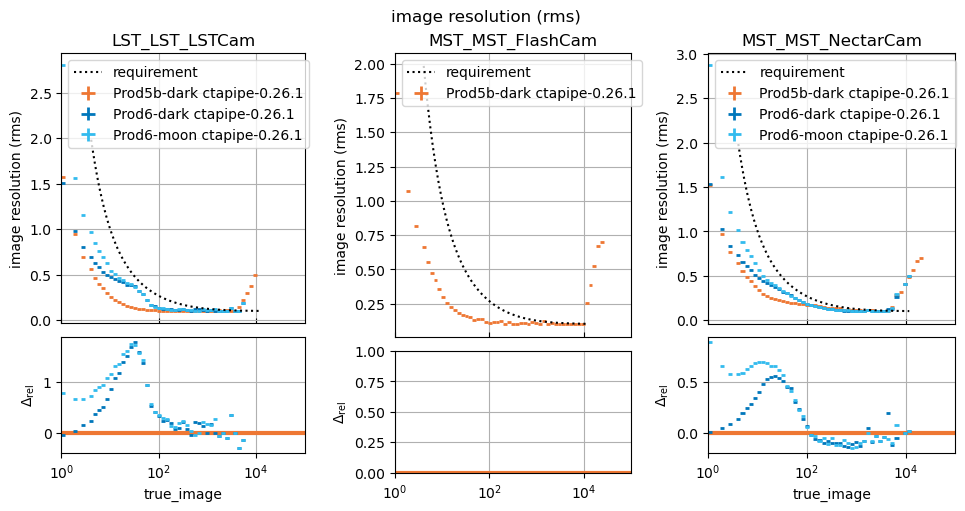
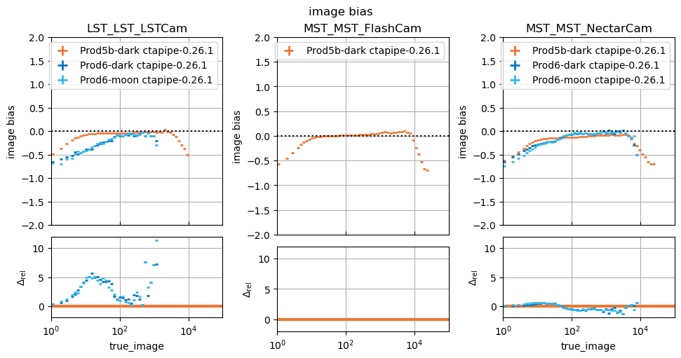
Now, we can run the study

_ = run_comparison_study(
    name="Compare pixel intensity resolution for different PRODs",
    experiment_names=experiment_names,
    benchmark_list=benchmark_list,
    experiments_path=EXPERIMENTS_PATH,  # the inputs
    studies_path=STUDIES_PATH,  # the outputs
)

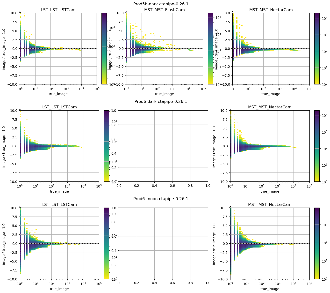
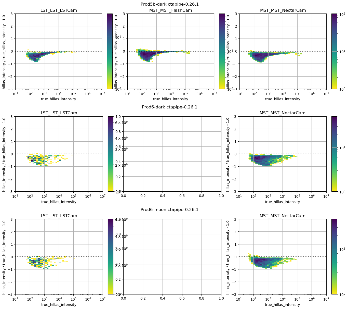
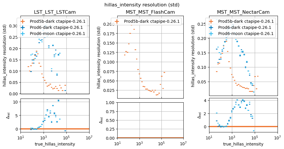
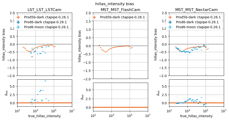
In this study, some plots are blank because the telescope type in question did not exist in the reference study, that is normal.

You can of course make more than one comparison study, using different input experiments, and include more than one benchmark. The outputs are stored in EXPERIMENTS_PATH in subdirectories named by the name of the study.

! tree $STUDIES_PATH

/Users/kkosack/testbench/studies
└── Compare pixel intensity resolution for different PRODs
    ├── dl1
    │   ├── hillas_intensity_bias.pdf
    │   ├── hillas_intensity_comparison_results.json
    │   ├── hillas_intensity_dispersion.pdf
    │   └── hillas_intensity_resolution.pdf
    ├── dl1_images
    │   ├── image_bias.pdf
    │   ├── image_comparison_results.json
    │   ├── image_dispersion.pdf
    │   └── image_resolution.pdf
    ├── metadata.json
    ├── study.dot
    └── study.dot.pdf

4 directories, 11 files

Troubleshooting

Inconsistent categories like telescope_type:

Sometimes, you want to make a study with new data, but where the name of the telecope type changed compared to old data. To get that to work, you can remap category names using rename_telescope_type(). You must however do that before you generate the metrics.

from datapipe_testbench import print_telescope_type_transforms, rename_telescope_type

# fix the case of "Cam":
rename_telescope_type("LST_LST_LSTcam", "LST_LST_LSTCam")

print_telescope_type_transforms()

*                 LST_LST_LSTcam -> LST_LST_LSTCam